Chapter 4: Challenges and Opportunities in Distributed Computing #
One of the critical tenants of life is tradeoffs. To gain one thing, you often lose another. With Distributed Computing, there is much to both gain and lose. Let’s talk through some of the keys concepts.
Learn what Debugging Python Code is in the following screencast.
Video Link: https://www.youtube.com/watch?v=BBCdU_3AI1E
Eventual Consistency #
The foundational infrastructure of the Cloud builds upon the concept of eventual consistency. This theory means that a relational database’s default behavior, for example, of strong consistency, is not needed in many Cloud Scale applications. For instance, if two users worldwide see a slightly different piece of text on a social media post and then 10 seconds later, a few more sentences change, and they become in sync, it is irrelevant to most humans viewing the post. Likewise, the social media company couldn’t care in the least in designing the application.
An excellent example of a product built around the Cloud Scale concept is Amazon DynamoDB. This database scales automatically, is key value-based, and is “eventually consistent.”
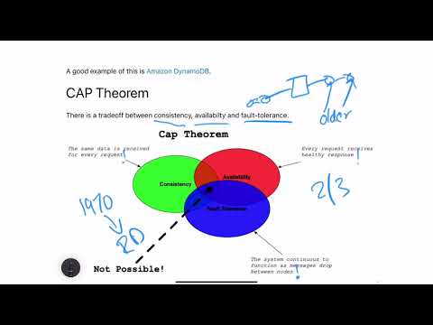
CAP Theorem #
There is a tradeoff between consistency, availability, and fault-tolerance according to the CAP Theorem. This theorem speaks to the statement you cannot gain one thing without losing another in Distributed Computing.

Learn what the CAP Theorem is in the following screencast.
Video Link: https://www.youtube.com/watch?v=hW6PL68yuB0
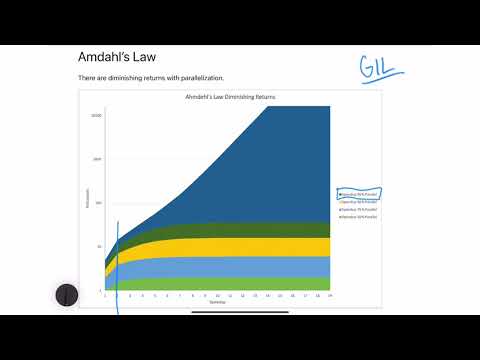
Amdahl’s Law #
Likewise, there are diminishing returns with parallelization. Just because more cores exist, it doesn’t mean they will be useful in all problems. Further, diminished efficiency occurs because most programs are not 100% parallel.
Learn what Amdahl’s Law is in the following screencast.
Video Link: https://www.youtube.com/watch?v=8pzBLcyTcR4
For each portion of the program that is not entirely parallel, the diminishing returns increase. Finally, some languages have critical flaws because they existed before multi-cores architectures were common. A great example of this is the Python language and the GIL (Global Interpreter Lock).
Learn about Concurrency in Python in the following screencast.

Video Link: https://www.youtube.com/watch?v=22BDJ4TIA5M
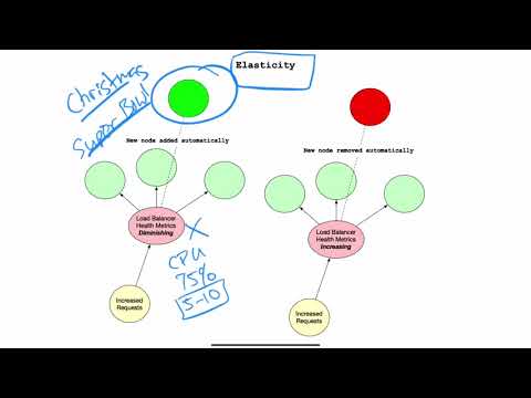
Elasticity #
Elasticity means the ability to adapt to a varying workload. In the world of Cloud Computing, this means you should only pay for what you use. It also means you can respond both to increased demand without failure, and you can scale down to reduce costs when the need diminishes.

Learn what Elasticity is in the following screencast.
Video Link: https://www.youtube.com/watch?v=HA2bh0oDMwo
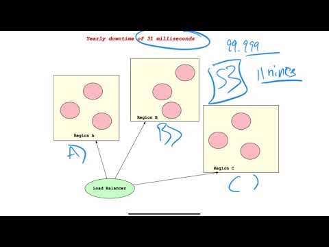
Highly Available #
Does the system always respond with a healthy response? An excellent example of a high availability system is Amazon S3. To build a HA (Highly Available) system, the Cloud provides the ability to architect against load balancers and regions.

Learn what Highly Available is in the following screencast.
Video Link: https://www.youtube.com/watch?v=UmAnxEOJSpM
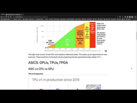
End of Moore’s Law #
Perhaps the best source to describe what is happening with chips is Dr. David Patterson, a professor at UC Berkeley and an architect for the TPU (Tensorflow Processing Unit).

The high-level version is that CPU clock speed is effectively dead. This “problem” opens up an opportunity for new solutions. These solutions involve both cloud computing, and also specialized chips called ASICs.
Learn about Moore’s Law in the following screencast.
Video Link: https://www.youtube.com/watch?v=adPvJpoj_tU
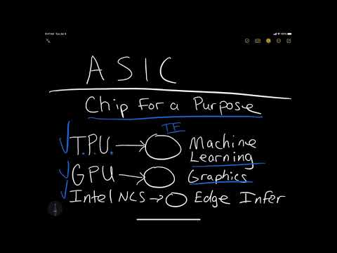
ASICS: GPUs, TPUs, FPGA #
Learn what an ASIC is in the following screencast.
Video Link: https://www.youtube.com/watch?v=SXLQ6ipVtxQ
ASIC vs CPU vs GPU #
TPU in Production

CPU

GPU

TPU

Sources: https://storage.googleapis.com/nexttpu/index.html
Using GPUs and JIT #
Learn how to do GPU programming is in the following screencast.

Video Link: https://www.youtube.com/watch?v=3dHJ00mAQAY
One of the easiest ways to use a Just in Time compiler (JIT) or a GPU is to use a library like numba and a hosted runtime like Google Colab.
Learn what Colab Pro is in the following screencast.
Video Link: https://www.youtube.com/watch?v=W8RcIP2-h7c
There is a step by step example of how to use these operations in the following notebook https://github.com/noahgift/cloud-data-analysis-at-scale/blob/master/GPU_Programming.ipynb. The main high-level takeaway is that a GPU runtime must exist. This example is available via Google Colab, but it could also live on a server somewhere or your workstation if it has an NVidia GPU.

Next up, you can install numba if not installed and double-check the CUDA .so libraries are available.
!pip install numba
!find / -iname 'libdevice'
!find / -iname 'libnvvm.so'
You should see something like this.
/usr/local/cuda-10.0/nvvm/libdevice
/usr/local/cuda-10.1/nvvm/libdevice
/usr/local/cuda-10.0/nvvm/lib64/libnvvm.so
/usr/local/cuda-10.1/nvvm/lib64/libnvvm.so
GPU Workflow #
A key concept in the GPU program is the following steps to code to the GPU from scratch.
- Create a Vectorized Function
- Move calculations to GPU memory
- Calculate on the GPU
- Move the Calculations back to the host
Here is a contrived example below that is available in this Google Colab Notebook.
from numba import (cuda, vectorize)
import pandas as pd
import numpy as np
from sklearn.preprocessing import MinMaxScaler
from sklearn.cluster import KMeans

from functools import wraps
from time import time

def real_estate_df():
    """30 Years of Housing Prices"""

    df = pd.read_csv("https://raw.githubusercontent.com/noahgift/real_estate_ml/master/data/Zip_Zhvi_SingleFamilyResidence.csv")
    df.rename(columns={"RegionName":"ZipCode"}, inplace=True)
    df["ZipCode"]=df["ZipCode"].map(lambda x: "{:.0f}".format(x))
    df["RegionID"]=df["RegionID"].map(lambda x: "{:.0f}".format(x))
    return df

def numerical_real_estate_array(df):
    """Converts df to numpy numerical array"""

    columns_to_drop = ['RegionID', 'ZipCode', 'City', 'State', 'Metro', 'CountyName']
    df_numerical = df.dropna()
    df_numerical = df_numerical.drop(columns_to_drop, axis=1)
    return df_numerical.values

def real_estate_array():
    """Returns Real Estate Array"""

    df = real_estate_df()
    rea = numerical_real_estate_array(df)
    return np.float32(rea)


@vectorize(['float32(float32, float32)'], target='cuda')
def add_ufunc(x, y):
    return x + y

def cuda_operation():
    """Performs Vectorized Operations on GPU"""

    x = real_estate_array()
    y = real_estate_array()

    print("Moving calculations to GPU memory")
    x_device = cuda.to_device(x)
    y_device = cuda.to_device(y)
    out_device = cuda.device_array(
        shape=(x_device.shape[0],x_device.shape[1]), dtype=np.float32)
    print(x_device)
    print(x_device.shape)
    print(x_device.dtype)

    print("Calculating on GPU")
    add_ufunc(x_device,y_device, out=out_device)

    out_host = out_device.copy_to_host()
    print(f"Calculations from GPU {out_host}")

cuda_operation()
Exercise-GPU-Coding #
- Topic: Go through colab example here
- Estimated time: 20-30 minutes
- People: Individual or Final Project Team
- Slack Channel: #noisy-exercise-chatter
- Directions:
- Part A: Get code working in colab
- Part B: Make your GPU or JIT code to speed up a project. Share in slack or create a technical blog post about it.
Summary #
This chapter covers the theory behind many Cloud Computing fundamentals, including Distributed Computing, CAP Theorem, Eventual Consistency, Amdahl’s Law, and Highly Available. It concludes with a hands-on example of doing GPU programming with CUDA in Python.