Chapter 5: Cloud Storage #
Unlike a desktop computer, the cloud offers many choices for storage. These options range from object storage to flexible network file systems. This chapter covers these different storage types as well as methods to deal with them.
Learn why Cloud Storage is essential in the following screencast.

Video Link: https://www.youtube.com/watch?v=4ZbPAzlmpcI
Cloud Storage Types #
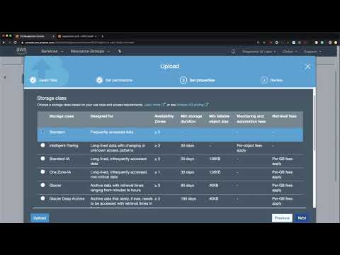
AWS is an excellent starting point to discuss the different storage options available in the cloud. You can see a list of the various storage options they provide here. Let’s address these options one by one.
Object Storage #
Amazon S3 is object storage with (11 9’s) of durability, meaning yearly downtime measures in milliseconds. It is ideal for storing large objects like files, images, videos, or other binary data. It is often the central location used in a Data Processing workflow. A synonym for an object storage system is a “Data Lake.”
Learn how to use Amazon S3 in the following screencast.
Video Link: https://www.youtube.com/watch?v=BlWfOMmPoPg
Learn what a Data Lake is in the following screencast.

Video Link: https://www.youtube.com/watch?v=fmsG91EgbBk
File Storage #
Many cloud providers now offer scalable, elastic File Systems. AWS provides the Amazon Elastic File System (EFS) and Google delivers the Filestore. These file systems offer high performance, fully managed file storage than can be mounted by multiple machines. These can serve as the central component of NFSOPS or Network File System Operations, where the file system stores the source code, the data, and the runtime.
Learn about Cloud Databases and Cloud Storage in the following screencast.

Video Link: https://www.youtube.com/watch?v=-68k-JS_Y88
Another option with Cloud Databases is to use serverless databases, such as AWS Aurora Serverless. Many databases in the Cloud work in a serverless fashion, including Google BigQuery and AWS DynamoDB. Learn to use AWS Aurora Serverless in the following screencast.

Video Link: https://www.youtube.com/watch?v=UqHz-II2jVA
Block Storage #
Block storage is similar to the hard drive storage on a workstation or laptop but virtualized. This virtualization allows for the storage to increase in size and performance. It also means a user can “snapshot” storage and use it for backups or operating system images. Amazon offers block storage through a service, Amazon Block Store, or EBS.
Other Storage #
There are various other storage types in the cloud, including backup systems, data transfer systems, and edge computing services like AWS Snowmobile can transfer 100 PB, yes petabyte, of data in a shipping container.
Data Governance #
What is Data Governance? It is the ability to “govern” the data. Who can access the data and what can they do with it are essential questions in data governance. Data Governance is a new emerging job title due to the importance of storing data securely in the cloud.
Learn about Data Governance in the following screencast.

*Video Link: https://www.youtube.com/watch?v=cCUiHBP7Bts
Learn about AWS Security in the following screencast.

Video Link: https://www.youtube.com/watch?v=I8FeP_FY9Rg
Learn about AWS Cloud Security IAM in the following screencast.

Video Link: https://www.youtube.com/watch?v=_Xf93LSCECI
Highlights of a Data Governance strategy include the following.
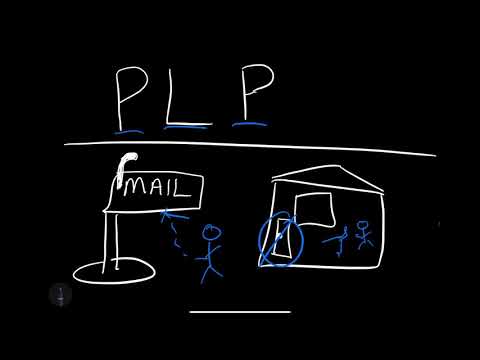
PLP (Principle of Least Privilage) #
Are you limiting the permissions by default vs. giving access to everything? This security principle is called the PLP, and it refers to only providing a user what they need. An excellent real-life analogy is not giving the mail delivery person access to your house, only giving them access to the mailbox.
Learn about PLP in the following screencast.
Video Link: https://www.youtube.com/watch?v=cIRa4P24sf4
Audit #
Is there an automated auditing system? How do you know when a security breach has occurred?
PII (Personally Identifiable Information) #
Is the system avoiding the storage of Personally Identifiable Information?
Data Integrity #
How are you ensuring that your data is valid and not corrupt? Would you know when it tampering occurred?
Disaster Recovery #
What is your disaster recovery plan, and how do you know it works? Did you test the backups through a reoccurring restore process?
Encrypt #
Do you encrypt data at transit and rest? Who has access to the encryption keys? Do you audit encryption events such as decryption of sensitive data?
Model Explainability #
Are you sure you could recreate the model? Do you know how it works, and is it explainable?
Data Drift #
Do you measure the “drift” of the data used to create Machine Learning models? Microsoft Azure has a good set of documentation about data drift that is a good starting point to learn about the concept.
Cloud Databases #
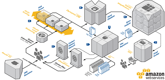
A big takeaway in the cloud is you don’t have to start with a relational database. The CTO of Amazon, Werner Vogel’s brings up some of the options available in the blog post A one size fits all database doesn’t serve anyone.
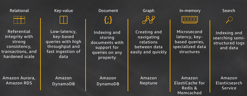 source: allthingsdistributed.com
Learn about one size doesn’t fit all in the following screencast.
Video Link: https://www.youtube.com/watch?v=HkequkfOIE8
Key-Value Databases #
An excellent example of a serverless key/value database is Dynamodb. Another famous example is MongoDB.
How could you query this type of database in pure Python?
def query_police_department_record_by_guid(guid):
    """Gets one record in the PD table by guid

    In [5]: rec = query_police_department_record_by_guid(
        "7e607b82-9e18-49dc-a9d7-e9628a9147ad"
        )

    In [7]: rec
    Out[7]:
    {'PoliceDepartmentName': 'Hollister',
     'UpdateTime': 'Fri Mar  2 12:43:43 2018',
     'guid': '7e607b82-9e18-49dc-a9d7-e9628a9147ad'}
    """

    db = dynamodb_resource()
    extra_msg = {"region_name": REGION, "aws_service": "dynamodb",
        "police_department_table":POLICE_DEPARTMENTS_TABLE,
        "guid":guid}
    log.info(f"Get PD record by GUID", extra=extra_msg)
    pd_table = db.Table(POLICE_DEPARTMENTS_TABLE)
    response = pd_table.get_item(
        Key={
            'guid': guid
            }
    )
    return response['Item']
Notice that there are only a couple of lines to retrieve data from the database without the logging code!
Learn to use AWS DynamoDB in the following screencast.
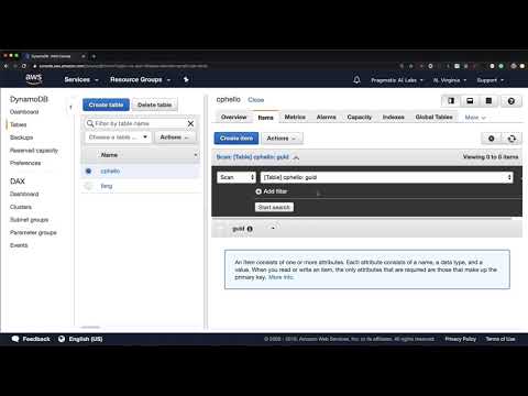
Video Link: https://www.youtube.com/watch?v=gTHE6X5fce8
Graph Databases #
Another specialty database is a Graph Database. When I was the CTO of a Sports Social Network, we used a Graph Database, Neo4J, to make social graph queries more feasible. It also allowed us to build products around data science more quickly.
Why Not Relational Databases instead of a Graph Database? #
Relationship data is not a good fit for relational databases. Here are some examples (ideas credit to Joshua Blumenstock-UC Berkeley).
-
Think about SQL query of social network used to select all third-degree connections of the individual.
- Imagine the number of joins needed.
-
Think about SQL query used to get a full social network of the individual.
- Imagine the number of recursive joins required.
Relational databases are good at representing one-to-many relationships, in which one table connects to multiple tables. Mimicking real-life relationships, like friends or followers in a social network, is much more complicated and a better fit for a Graph Database.
AWS Neptune #
The Amazon Cloud also has a Graph database called Amazon Neptune, which has similar properties to Neo4J.

Neo4j #
You can learn more about Neo4j by experimenting in the sandbox they provide. The following graph tutorial is HEAVILY based on their official documentation, which you can find in the link below.
Graph Database Facts #
Let’s dive into some of the critical Graph Database facts.
Graph Database can store:
- Nodes - graph data records
- Relationships - connect nodes
- Properties - named data values
Simplest Graph #
The Simplest Graph is as follows.
- One node
- Has some properties
- Start by drawing a circle for the node
- Add the name, Emil
- Note that he is from Sweden
- Nodes are the name for data records in a graph
- Data is stored as Properties
- Properties are simple name/value pairs

Labels #
“Nodes” group together by applying a Label to each member. In our social graph, we’ll label each node that represents a Person.
- Apply the label “Person” to the node we created for Emil
- Color “Person” nodes red
- A node can have zero or more labels
- Labels do not have any properties

More Nodes #
Like any database, storing data in Neo4j can be as simple as adding more records. We’ll add a few more nodes:
- Emil has a Klout score of 99
- Johan, from Sweden, who is learning to surf
- Ian, from England, who is an author
- Rik, from Belgium, has a cat named Orval
- Allison, from California, who surfs
- Similar nodes can have different properties
- Properties can be strings, numbers, or booleans
- Neo4j can store billions of nodes

Relationships #
The real power of Neo4j is in connected data. To associate any two nodes, add a Relationship that describes how the records are related.
In our social graph, we simply say who KNOWS whom:
- Emil KNOWS Johan and Ian
- Johan KNOWS Ian and Rik
- Rik and Ian KNOWS Allison
- Relationships always have direction
- Relationships still have a type
- Relationships form patterns of data

Relationship Properties #
In a property graph, relationships are data records that can also** contain properties**. Looking more closely at Emil’s relationships, note that:
- Emil has known Johan since 2001
- Emil rates Ian 5 (out of 5)
- Everyone else can have similar relationship properties

Key Graph Algorithms (With neo4j) #
An essential part of graph databases is the fact that they have different descriptive statistics. Here are these unique descriptive statistics.
-
Centrality - What are the most critical nodes in the network? PageRank, Betweenness Centrality, Closeness Centrality
-
Community detection - How can the graph be partitioned? Union Find, Louvain, Label Propagation, Connected Components
-
Pathfinding - What are the shortest paths or best routes available given the cost? Minimum Weight Spanning Tree, All Pairs- and Single Source- Shortest Path, Dijkstra
Let’s take a look at the Cypher code to do this operation.
CALL dbms.procedures()
YIELD name, signature, description
WITH * WHERE name STARTS WITH "algo"
RETURN *
Russian Troll Walkthrough [Demo] #
One of the better sandbox examples on the Neo4J website is the Russian Troll dataset. To run through an example, run this cipher code in their sandbox.
:play https://guides.neo4j.com/sandbox/twitter-trolls/index.html
Finding top Trolls with Neo4J #
You can proceed to find the “trolls”, i.e., foreign actors causing trouble in social media, in the example below.
The list of prominent people who tweeted out links from the account, @Ten_GOP, which Twitter shut down in August, includes political figures such as Michael Flynn and Roger Stone, celebrities such as Nicki Minaj and James Woods, and media personalities such as Anne Coulter and Chris Hayes. Note that at least two of these people were also convicted of a Felony and then pardoned, making the data set even more enjoyable.
A screenshot of the Neo4J interface for the phrase “thanks obama.”

Pagerank score for Trolls #
Here is a walkthrough of code in a colab notebook you can reference called social network theory.
def enable_plotly_in_cell():
  import IPython
  from plotly.offline import init_notebook_mode
  display(IPython.core.display.HTML('''
        <script src="/static/components/requirejs/require.js"></script>
  '''))
  init_notebook_mode(connected=False)
The trolls export from Neo4j and they load into Pandas.
import pandas as pd
import numpy as np

df = pd.read_csv("https://raw.githubusercontent.com/noahgift/essential_machine_learning/master/pagerank_top_trolls.csv")
df.head()

Next up, the data graphs with Plotly.
import plotly.offline as py
import plotly.graph_objs as go

from plotly.offline import init_notebook_mode
enable_plotly_in_cell()
init_notebook_mode(connected=False)


fig = go.Figure(data=[go.Scatter(
    x=df.pagerank,
    text=df.troll,
    mode='markers',
    marker=dict(
        color=np.log(df.pagerank),
        size=df.pagerank*5),
)])
py.iplot(fig, filename='3d-scatter-colorscale')

Top Troll Hashtags
import pandas as pd
import numpy as np

df2 = pd.read_csv("https://raw.githubusercontent.com/noahgift/essential_machine_learning/master/troll-hashtag.csv")
df2.columns = ["hashtag", "num"]
df2.head()

Now plot these troll hashtags.
import plotly.offline as py
import plotly.graph_objs as go

from plotly.offline import init_notebook_mode
enable_plotly_in_cell()
init_notebook_mode(connected=False)


fig = go.Figure(data=[go.Scatter(
    x=df.pagerank,
    text=df2.hashtag,
    mode='markers',
    marker=dict(
        color=np.log(df2.num),
        size=df2.num),
)])
py.iplot(fig)
You can see these trolls love to use the hashtag #maga.

Graph Database References #
The following are additional references.
The Three “V’s” of Big Data: Variety, Velocity, and Volume #
There are many ways to define Big Data. One way of describing Big Data is that it is too large to process on your laptop. Your laptop is not the real world. Often it comes as a shock to students when they get a job in the industry that the approach they learned in school doesn’t work in the real world!
Learn what Big Data is in the following screencast.

Video Link: https://www.youtube.com/watch?v=2-MrUUj0E-Q
Another method is the Three “V’s” of Big Data: Variety, Velocity, and Volume.

Learn the three V’s of Big Data is in the following screencast.
Video Link: https://www.youtube.com/watch?v=qXBcDqSy5GY
Variety #
Dealing with many types of data is a massive challenge in Big Data. Here are some examples of the types of files dealt with in a Big Data problem.
- Unstructured text
- CSV files
- binary files
- big data files: Apache Parquet
- Database files
- SQL data
Velocity #
Another critical problem in Big Data is the velocity of the data. Some questions to include the following examples. Are data streams written at 10’s of thousands of records per second? Are there many streams of data written at once? Does the velocity of the data cause performance problems on the nodes collecting the data?
Volume #
Is the actual size of the data more extensive than what a workstation can handle? Perhaps your laptop cannot load a CSV file into the Python pandas package. This problem could be Big Data, i.e., it doesn’t work on your laptop. One Petabyte is Big Data, and 100 GB could be big data depending on its processing.
Batch vs. Streaming Data and Machine Learning #
One critical technical concern is Batch data versus Stream data. If data processing occurs in a Batch job, it is much easier to architect and debug Data Engineering solutions. If the data is streaming, it increases the complexity of architecting a Data Engineering solution and limits its approaches.
Impact on ML Pipeline #
One aspect of Batch vs. Stream is that there is more control of model training in batch (can decide when to retrain). On the other hand, continuously retraining the model could provide better prediction results or worse results. For example, did the input stream suddenly get more users or fewer users? How does an A/B testing scenario work?
Batch #
What are the characteristics of Batch data?
- Data is batched at intervals
- Simplest approach to creating predictions
- Many Services on AWS Capable of Batch Processing including, AWS Glue, AWS Data Pipeline, AWS Batch, and EMR.
Streaming #
What are the characteristics of Streaming data?
- Continuously polled or pushed
- More complex method of prediction
- Many Services on AWS Capable of Streaming, including Kinesis, IoT, and Spark EMR.
Cloud Data Warehouse #
The advantage of the cloud is infinite compute and infinite storage. Cloud-native data warehouse systems also allow for serverless workflows that can directly integrate Machine Learning on the data lake. They are also ideal for developing Business Intelligence solutions.
GCP BigQuery #
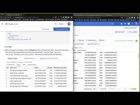
There is a lot to like about GCP BigQuery. It is serverless, it has integrated Machine Learning, and it is easy to use. This next section has a walkthrough of a k-means clustering tutorial.
The interface, when queried, intuitively gives back results. A key reason for this is the use of SQL and the direct integration with both Google Cloud and Google Data Studio

Learn to use Google BigQuery in the following screencast.
Video Link: https://www.youtube.com/watch?v=eIec2DXqw3Q
Even better, you can directly train Machine Learning models using a SQL statement. This workflow shows an emerging trend with Cloud Database services in that they let you both query the data and train the model. In this example, the kmeans section is where the magic happens.
CREATE OR REPLACE MODEL
  bqml_tutorial.london_station_clusters OPTIONS(model_type='kmeans',
    num_clusters=4) AS
WITH
  hs AS (
  SELECT
    h.start_station_name AS station_name,
  IF
    (EXTRACT(DAYOFWEEK
      FROM
        h.start_date) = 1
      OR EXTRACT(DAYOFWEEK
      FROM
        h.start_date) = 7,
      "weekend",
      "weekday") AS isweekday,
    h.duration,
    ST_DISTANCE(ST_GEOGPOINT(s.longitude,
        s.latitude),
      ST_GEOGPOINT(-0.1,
        51.5))/1000 AS distance_from_city_center
  FROM
    `bigquery-public-data.london_bicycles.cycle_hire` AS h
  JOIN
    `bigquery-public-data.london_bicycles.cycle_stations` AS s
  ON
    h.start_station_id = s.id
  WHERE
    h.start_date BETWEEN CAST('2015-01-01 00:00:00' AS TIMESTAMP)
    AND CAST('2016-01-01 00:00:00' AS TIMESTAMP) ),
  stationstats AS (
  SELECT
    station_name,
    isweekday,
    AVG(duration) AS duration,
    COUNT(duration) AS num_trips,
    MAX(distance_from_city_center) AS distance_from_city_center
  FROM
    hs
  GROUP BY
    station_name, isweekday)
SELECT
  * EXCEPT(station_name, isweekday)
FROM
  stationstats
Finally, when the k-means clustering model trains, the evaluation metrics appear as well in the console.

Often a meaningful final step is to take the result and then export it to their Business Intelligence (BI) tool, data studio.

The following is an excellent example of what a cluster visualization could look like in Google Big Query exported to Google Data Studio.

You can view the report using this direct URL.
Summary of GCP BigQuery #
In a nutshell, GCP BigQuery is a useful tool for Data Science and Business Intelligence. Here are the key features.
- Serverless
- Large selection of Public Datasets
- Integrated Machine Learning
- Integration with Data Studio
- Intuitive
- SQL based
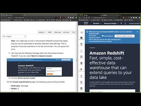
AWS Redshift #
AWS Redshift is a Cloud data warehouse designed by AWS. The key features of Redshift include the ability to query exabyte data in seconds through the columnar design. In practice, this means excellent performance regardless of the size of the data.
Learn to use AWS Redshift in the following screencast.
Video Link: https://www.youtube.com/watch?v=vXSH24AJzrU
Key actions in a Redshift Workflow #
In general, the key actions are as described in the Redshift getting started guide. These are the critical steps to setup a workflow.
-
Cluster Setup
-
IAM Role configuration (what can role do?)
-
Setup Security Group (i.e. open port 5439)
-
Setup Schema
  create table users(
  userid integer not null distkey sortkey,
  username char(8),
- Copy data from S3
  copy users from 's3://awssampledbuswest2/tickit/allusers_pipe.txt'
  credentials 'aws_iam_role=<iam-role-arn>'
  delimiter '|' region 'us-west-2';
- Query
  SELECT firstname, lastname, total_quantity
  FROM
  (SELECT buyerid, sum(qtysold) total_quantity
  FROM  sales
  GROUP BY buyerid
  ORDER BY total_quantity desc limit 10) Q, users
  WHERE Q.buyerid = userid
  ORDER BY Q.total_quantity desc;
Summary of AWS Redshift #
The high-level takeaway for AWS Redshift is the following.
- Mostly managed
- Deep Integration with AWS
- Columnar
- Competitor to Oracle and GCP Big Query
- Predictable performance on massive datasets
Summary #
This chapter covers storage, including object, block, filesystem, and Databases. A unique characteristic of Cloud Computing is the ability to use many tools at once to solve a problem. This advantageous trait is heavily at play with the topic of Cloud Storage and Cloud Databases.